Not quite, mainly because so many other libraries have covered this quite well. Let’s look at some examples:
Using Base-R
states <- read_csv("us-states.csv")
states %>% select(cases, deaths) %>% summary()

     cases             deaths
 Min.   :      1   Min.   :    0
 1st Qu.:  10205   1st Qu.:  233
 Median :  78464   Median : 1570
 Mean   : 248857   Mean   : 5022
 3rd Qu.: 304485   3rd Qu.: 5906
Max. :3795820 Max. :63544 psych packagelibrary(psych)
states %>% select(cases, deaths) %>% psych::describe()
vars n mean sd median trimmed mad min max
cases 1 25369 248857.2 459490.12 78464 147409.31 113596.81 1 3795820
deaths 2 25369 5022.3 8748.31 1570 2944.01 2286.17 0 63544
range skew kurtosis se
cases 3795819 4.07 21.58 2884.86
deaths 63544 3.27 12.93 54.93Hmisc packagestates %>% select(cases, deaths) %>% Hmisc::describe()
.
2 Variables 25369 Observations
--------------------------------------------------------------------------------
cases
n missing distinct Info Mean Gmd .05 .10
25369 0 21528 1 248857 354122 82.4 896.8
.25 .50 .75 .90 .95
10205.0 78464.0 304485.0 665750.6 987267.6
lowest : 1 2 3 4 5
highest: 3791972 3793055 3794235 3795063 3795820
--------------------------------------------------------------------------------
deaths
n missing distinct Info Mean Gmd .05 .10
25369 0 9545 1 5022 7115 2 16
.25 .50 .75 .90 .95
233 1570 5906 14179 22162
lowest : 0 1 2 3 4, highest: 63287 63345 63393 63423 63544
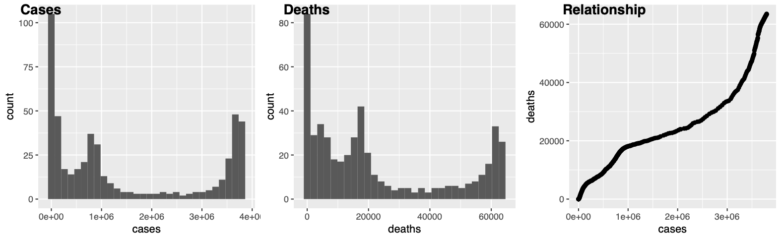
--------------------------------------------------------------------------------ggplot2 can draw individual plots but in order to put many plots together in a multi-panel figure, we need to rely on external libraries. Here are a couple of examples. First let’s make some individual plots.plot1 <- states %>% filter(state == "California") %>% ggplot() + geom_histogram(aes(x=cases))
plot2 <- states %>% filter(state == "California") %>% ggplot() + geom_histogram(aes(x=deaths))
plot3 <- states %>% filter(state == "California") %>% ggplot() + geom_point(aes(x=cases, y=deaths))Now get the following libraries:
ggpubr, cowplotggpubrlibrary(ggpubr)
ggarrange(plot1, plot2, plot3, labels=c("Cases", "Deaths", "Relationship"), ncol=3, nrow=1)
ggsave("combined_ggarrange.pdf")cowplotlibrary(cowplot)
plot_grid(plot1, plot2, plot3, labels=c("Cases", "Deaths", "Relationship"), ncol=3, nrow=1)
ggsave("combined_cowplot.pdf")Load iris, a built in data set in R.
Using psych package, calculate summary statistics on only the numerical data portion in iris
Create four histograms for each of the four numerical variables and store them into R objects
Using the ggpubr package, create a multi panel plot and use ggsave to write it to a file.