December 3, 2021
The file conversion will be similar to how we did it for Structure using PGDSpider. We need the following files:
Population file (ruber.pop)
PGDSpider template file (vcf2bscan.spid)
Input VCF file (ruber_reduced_ref.vcf)
You can copy these files from: /project/inbre-train/2021_popgen_wkshp/data/Bayescan. Copy all files from this folder.
cd /path/to/your/gscratch/folder

cp /project/inbre-train/2021_popgen_wkshp/data/Bayescan/data/* .


ls -lh

-rw-rw-r-- 1 vchhatre  670 Dec  2 10:56 crovir.pop
-rw-r--r-- 1 vchhatre  336 Dec  2 10:57 vcf2bscan.sh
-rw-r--r-- 1 vchhatre 1.5K Dec  2 10:57 vcf2bscan.spid
-rw-rw-r-- 1 vchhatre 2.6M Dec 2 10:58 ruber_reduced_ref.vcfYou might recall that the VCF file contains some loci with more than 2 alleles. We need to exclude those loci from further analysis because they violate the assumptions of the method (Bayescan) we are about to use.
module load gcc swset perl vcftools

vcftools --vcf ruber_reduced_ref.vcf

VCFtools - 0.1.14
(C) Adam Auton and Anthony Marcketta 2009

Parameters as interpreted:
    --vcf ruber_reduced_ref.vcf

After filtering, kept 33 out of 33 Individuals
After filtering, kept 4562 out of a possible 4562 Sites
Run Time = 0.00 seconds
vcftools --vcf ruber_reduced_ref.vcf --min-alleles 2 --max-alleles 2

VCFtools - 0.1.14
(C) Adam Auton and Anthony Marcketta 2009

Parameters as interpreted:
    --vcf ruber_reduced_ref.vcf
    --max-alleles 2
    --min-alleles 2

After filtering, kept 33 out of 33 Individuals
After filtering, kept 4502 out of a possible 4562 Sites
Run Time = 0.00 seconds
vcftools --vcf ruber_reduced_ref.vcf --min-alleles 2 --max-alleles 2 --recode --out ruber_4502snp

VCFtools - 0.1.14
(C) Adam Auton and Anthony Marcketta 2009

Parameters as interpreted:
    --vcf ruber_reduced_ref.vcf
    --max-alleles 2
    --min-alleles 2
    --out ruber_4502snp
    --recode

After filtering, kept 33 out of 33 Individuals
Outputting VCF file...
After filtering, kept 4502 out of a possible 4562 Sites
Run Time = 0.00 seconds
vcftools --vcf ruber_4502snp.recode.vcf

VCFtools - 0.1.14
(C) Adam Auton and Anthony Marcketta 2009

Parameters as interpreted:
    --vcf ruber_4502snp.recode.vcf

After filtering, kept 33 out of 33 Individuals
After filtering, kept 4502 out of a possible 4502 Sites
Run Time = 0.00 seconds
mv ruber_4502snp.recode.vcf ruber_4502snp.vcfvim crovir.pop
SD_Field_0201 north
SD_Field_0255 south
SD_Field_0386 south
SD_Field_0491 south
SD_Field_0492 admixed
SD_Field_0493 south
SD_Field_0557 south
SD_Field_0598 admixed
SD_Field_0599 south
SD_Field_0642 admixed
SD_Field_0666 admixed
SD_Field_0983 north
SD_Field_1079 south
SD_Field_1205 north
SD_Field_1220 south
SD_Field_1225 south
SD_Field_1226 south
SD_Field_1381 north
SD_Field_1878 north
SD_Field_1880 north
SD_Field_1899 north
SD_Field_1961 south
SD_Field_1988 south
SD_Field_1991 south
SD_Field_2127 north
SD_Field_2287 admixed
SD_Field_2383 south
SD_Field_2427 south
SD_Field_2789 north
SD_Field_2914 south
SD_Field_2968 north
SD_Field_3027 north
SD_Field_3124 northvim vcf2bscan.spid# VCF Parser questions
PARSER_FORMAT=VCF
# Only output SNPs with a phred-scaled quality of at least:
VCF_PARSER_QUAL_QUESTION=
# Select population definition file:
VCF_PARSER_POP_FILE_QUESTION=
# What is the ploidy of the data?
VCF_PARSER_PLOIDY_QUESTION=DIPLOID
# Do you want to include a file with population definitions?
VCF_PARSER_POP_QUESTION=true
# Output genotypes as missing if the phred-scale genotype quality is below:
VCF_PARSER_GTQUAL_QUESTION=
# Do you want to include non-polymorphic SNPs?
VCF_PARSER_MONOMORPHIC_QUESTION=FALSE
# Only output following individuals (ind1, ind2, ind4, ...):
VCF_PARSER_IND_QUESTION=
# Only input following regions (refSeqName:start:end, multiple regions: whitespace separated):
VCF_PARSER_REGION_QUESTION=
# Output genotypes as missing if the read depth of a position for the sample is below:
VCF_PARSER_READ_QUESTION=
# Take most likely genotype if "PL" or "GL" is given in the genotype field?
VCF_PARSER_PL_QUESTION=false
# Do you want to exclude loci with only missing data?
VCF_PARSER_EXC_MISSING_LOCI_QUESTION=true
# GESTE / BayeScan Writer questions
WRITER_FORMAT=GESTE_BAYE_SCAN
# Specify which data type should be included in the GESTE / BayeScan file (GESTE / BayeScan can only analyze one data type per file):
GESTE_BAYE_SCAN_WRITER_DATA_TYPE_QUESTION=SNPvcf2bscan.sh Scriptvim vcf2bscan.sh#!/bin/bash
pgdspider -inputfile \
-inputformat VCF \
-outputfile \
-outputformat GESTE_BAYE_SCAN \
-spid vcf2bscan.spidThen run the script:
sbatch vcf2bscan.shLet’s take a look at the ruber.bayescan file
vim ruber.bayescan[loci]=4502
[populations]=3
[pop]=1
1 24 2 16 8
2 24 2 0 24
3 24 2 23 1
4 24 2 24 0
5 18 2 0 18
6 8 2 0 8
7 4 2 1 3
8 24 2 0 24
9 24 2 24 0
10 24 2 4 20
11 24 2 13 11
12 24 2 1 23
13 2 2 0 2
14 22 2 0 22
15 24 2 0 24
16 10 2 10 0
17 20 2 7 13
18 22 2 19 3This is a partial view of the file. The fields are as follows:
The number in the third column must always be 2. Our filtering of the vcf above was done precisely for this purpose. Still, you can once again verify that this number is 2 throughout:
sed -n 6,4507p ruber.bayescan | cut -f3 | sort | uniq -c

4502 2module load gcc swset bayescan
bayescan -h
---------------------------
| BayeScan 2.0 usage: |
---------------------------
-help Prints this help
---------------------------
| Input |
---------------------------
alleles.txt Name of the genotypes data input file
-d discarded Optional input file containing list of loci to discard
-snp Use SNP genotypes matrix
---------------------------
| Output |
---------------------------
-od . Output file directory, default is the same as program file
-o alleles Output file prefix, default is input file without the extension
-fstat Only estimate F-stats (no selection)
-all_trace Write out MCMC trace also for alpha paremeters (can be a very large file)
---------------------------
| Parameters of the chain |
---------------------------
-threads n Number of threads used, default is number of cpu available
-n 5000 Number of outputted iterations, default is 5000
-thin 10 Thinning interval size, default is 10
-nbp 20 Number of pilot runs, default is 20
-pilot 5000 Length of pilot runs, default is 5000
-burn 50000 Burn-in length, default is 50000
---------------------------
| Parameters of the model |
---------------------------
-pr_odds 10 Prior odds for the neutral model, default is 10
-lb_fis 0 Lower bound for uniform prior on Fis (dominant data), default is 0
-hb_fis 1 Higher bound for uniform prior on Fis (dominant data), default is 1
-beta_fis Optional beta prior for Fis (dominant data, m_fis and sd_fis need to be set)
-m_fis 0.05 Optional mean for beta prior on Fis (dominant data with -beta_fis)
-sd_fis 0.01 Optional std. deviation for beta prior on Fis (dominant data with -beta_fis)
-aflp_pc 0.1 Threshold for the recessive genotype as a fraction of maximum band intensity, default is 0.1
---------------------------
| Output files |
---------------------------
-out_pilot Optional output file for pilot runs
-out_freq Optional output file for allele frequenciesHere are the parameters we will be using:
-snp indicates that we are using SNP data-od specifies output directory.-threads n We will use 16 threads-n 5000 Similar to structure MCMC. We will set this to 20000-thin 10 Keep this as is-nbp 20 Keep as is-pilot 5000 This is fine as well-burn 50000 Keep as is-pr_odds 10 Change this to 1000. 10 is too high a number-out_freq Obtain output allele frequencies in addition to selection scanLet’s make a script:
vim run_bayescan.sh
module load gcc swset bayescan/2.1


bayescan ruber.bayescan -snp \
    -od ruber_output    \
    -threads 16 \
    -n 5000 \
    -thin 10    \
    -nbp 20 \
    -pilot 5000 \
    -burn 50000 \
    -pr_odds 1000   \
    -out_freq
mkdir ruber_output

sbatch run_bayescan.shBayescan outputs several files depending upon parameters selected during the run. You will see the following files in the results folder:
cd ruber_output

ls -lh

-rw-rw-r-- 1 vchhatre 380K Dec  2 14:38 ruber.baye_Verif.txt
-rw-rw-r-- 1 vchhatre  601 Dec  2 15:17 ruber.baye_AccRte.txt
-rw-rw-r-- 1 vchhatre 252K Dec  2 15:17 ruber.baye.sel
-rw-rw-r-- 1 vchhatre 228K Dec 2 19:16 ruber.baye_fst.txt.baye_fst.txt has most of the results for selection scan. Let’s take a look.vim ruber.baye_fst.txtAdd a name for the first column. Call it loci.
Then replace multiple spaces between columns by a single tab
:%s/\s\+/ /g
:%s/ /\t/g
:wqmodule load gcc swset r
Rbscan <- read.table("ruber.baye_fst.txt", header=T)
head(bscan)
locus prob log10.PO. qval alpha fst
1 1 0.00080016 -3.09648 0.998716 -0.00014427 0.32671
2 2 0.00080016 -3.09650 0.998720 -0.00025595 0.32669
3 3 0.00100020 -2.99950 0.998560 -0.00021504 0.32671
4 4 0.00080016 -3.09650 0.998720 -0.00038205 0.32668
5 5 0.00060012 -3.22150 0.998840 -0.00012257 0.32671
6 6 0.00060012 -3.22150 0.998840 0.00085670 0.32693Here: - prob is the posterior probability of selection acting on a locus - log10.PO. is the log10 of the posterior odds of the model testing for selection. The value in this column is set to 1000 when the posterior probability is 1. - alpha is a coefficient indicating the strength and direction of selection. Positive values indicate diversifying selection and negative values, purifying selection. - qval is the multiple testing p-value obtained after testing each locus for selection.
qvalue should be very small. Let’s check the range of these values.range(bscan$qval)
[1] 0.90958 0.99897This indicates that there are no loci that can be considered candidates for selection.
It’s possible that the prior odds we set (pr_odds=1000) is too small. Maybe we should increase those odds by an order of magnitude (say 100). We can rerun the analysis by making two small changes to the script:
vim run_bayescan.sh-pr_odds 100
-od ruber_output_prior100mkdir ruber_output_prior100
sbatch run_bayescan.shBecause our current data set does not seem to have any outliers showing extreme allele frequency differences, we will switch to a different data set for illustration purposes. You can find this data inside the data/ folder for this week on Github.
cd Bayescan

wget https://github.com/wyoibc/popgen_workshop/tree/master/week5/selection/data/test_baye_fst.txt
test <- read.table("test.baye_fst.txt", header=T)

head(test)

        prob  log10.PO.     qval       alpha      fst
1 0.00000000 -1000.0000 0.997644  0.0000e+00 0.022319
2 0.00000000 -1000.0000 0.997640  0.0000e+00 0.022319
3 0.00000000 -1000.0000 0.997640  0.0000e+00 0.022319
4 0.00020004    -3.6988 0.994060  1.5625e-04 0.022324
5 0.00020004    -3.6988 0.994060 -5.8927e-05 0.022318
6 0.00000000 -1000.0000 0.997640 0.0000e+00 0.022319dim(test)
[1] 107309 5range(test$qval)
[1] 0.000000 0.997644library(ggplot2)
ggplot(data=test) + geom_histogram(aes(x=qval), binwidth=0.01)sum(test$qval < 0.05)
[1] 222sum(test$qval < 0.001)
145subset(test, qval < 0.001)
prob log10.PO. qval alpha fst
1566 0.9918 2.0825 4.6531e-04 1.7248 0.114760
1568 0.9882 1.9229 9.2708e-04 1.7285 0.115480
1700 0.9892 1.9618 8.5156e-04 1.7330 0.115720
1702 0.9964 2.4420 2.5378e-04 1.7605 0.117830
3159 0.9912 2.0516 5.8297e-04 1.6601 0.108270
3192 1.0000 1000.0000 0.0000e+00 1.9705 0.138040
6013 1.0000 1000.0000 0.0000e+00 2.8917 0.278710
6650 1.0000 1000.0000 0.0000e+00 2.0830 0.153020
6931 0.9996 3.3977 2.2613e-05 2.2409 0.174450
12697 1.0000 1000.0000 0.0000e+00 1.8961 0.131350
14156 1.0000 1000.0000 0.0000e+00 2.1488 0.159040
14171 1.0000 1000.0000 0.0000e+00 2.2797 0.176420
14201 0.9998 3.6988 9.0108e-06 1.7465 0.116600
14954 1.0000 1000.0000 0.0000e+00 2.6822 0.239490
18125 1.0000 1000.0000 0.0000e+00 2.1727 0.164620
18300 1.0000 1000.0000 0.0000e+00 1.9129 0.131840
18322 1.0000 1000.0000 0.0000e+00 1.6018 0.101940
18394 1.0000 1000.0000 0.0000e+00 1.8083 0.121450
18396 1.0000 1000.0000 0.0000e+00 1.8114 0.121840
24167 1.0000 1000.0000 0.0000e+00 2.2193 0.167970
24395 1.0000 1000.0000 0.0000e+00 1.8848 0.128070
26773 1.0000 1000.0000 0.0000e+00 1.7408 0.114220
27418 1.0000 1000.0000 0.0000e+00 2.4339 0.196440
27423 1.0000 1000.0000 0.0000e+00 2.0684 0.148980
31272 1.0000 1000.0000 0.0000e+00 2.4578 0.203560
34814 1.0000 1000.0000 0.0000e+00 1.8200 0.122140
34830 1.0000 1000.0000 0.0000e+00 1.8360 0.124590
36086 1.0000 1000.0000 0.0000e+00 1.8240 0.121930
39272 1.0000 1000.0000 0.0000e+00 3.5160 0.396580
39876 1.0000 1000.0000 0.0000e+00 1.9194 0.133520
39889 1.0000 1000.0000 0.0000e+00 1.8886 0.130840
39890 0.9994 3.2215 3.7296e-05 1.8842 0.130450
39910 1.0000 1000.0000 0.0000e+00 1.8167 0.123000
42021 0.9974 2.5838 2.0762e-04 2.3243 0.188730
42351 1.0000 1000.0000 0.0000e+00 2.1141 0.154780
43349 0.9984 2.7951 1.0955e-04 3.3251 0.364780
43516 1.0000 1000.0000 0.0000e+00 1.7734 0.118360
43760 1.0000 1000.0000 0.0000e+00 1.8764 0.129290
43771 1.0000 1000.0000 0.0000e+00 2.1364 0.159980
43775 1.0000 1000.0000 0.0000e+00 2.1471 0.161570
43778 1.0000 1000.0000 0.0000e+00 2.1421 0.160850
45050 0.9998 3.6988 9.0108e-06 1.7325 0.114640
45053 0.9926 2.1275 4.0884e-04 1.6045 0.103530
46669 1.0000 1000.0000 0.0000e+00 1.8368 0.126170
46861 0.9986 2.8532 8.5501e-05 1.8843 0.130930
48480 1.0000 1000.0000 0.0000e+00 1.8787 0.129220
49162 1.0000 1000.0000 0.0000e+00 1.7046 0.111360
50013 1.0000 1000.0000 0.0000e+00 1.8834 0.128270
51912 1.0000 1000.0000 0.0000e+00 1.7774 0.118170
51917 1.0000 1000.0000 0.0000e+00 1.8019 0.120470
51920 1.0000 1000.0000 0.0000e+00 1.8123 0.121500
51936 0.9976 2.6187 1.8935e-04 1.5646 0.099173
53114 1.0000 1000.0000 0.0000e+00 1.7699 0.117520
54009 1.0000 1000.0000 0.0000e+00 2.6047 0.228290
54544 0.9990 2.9995 6.3947e-05 1.7931 0.120470
57035 1.0000 1000.0000 0.0000e+00 2.5100 0.212890
58556 1.0000 1000.0000 0.0000e+00 2.1872 0.168830
58559 0.9998 3.6988 9.0108e-06 1.9893 0.144050
59329 1.0000 1000.0000 0.0000e+00 1.6750 0.108510
59877 1.0000 1000.0000 0.0000e+00 1.8073 0.121550
59878 1.0000 1000.0000 0.0000e+00 1.8124 0.122040
61797 0.9998 3.6988 9.0108e-06 2.4507 0.205690
66090 0.9998 3.6988 9.0108e-06 1.8892 0.131120
66817 0.9992 3.0965 5.6210e-05 1.7872 0.120200
70550 1.0000 1000.0000 0.0000e+00 2.5538 0.215940
70551 1.0000 1000.0000 0.0000e+00 4.2592 0.559140
70553 1.0000 1000.0000 0.0000e+00 3.1107 0.311520
70554 1.0000 1000.0000 0.0000e+00 3.0005 0.290330
70556 1.0000 1000.0000 0.0000e+00 2.2939 0.177830
70557 1.0000 1000.0000 0.0000e+00 4.0050 0.502850
70561 1.0000 1000.0000 0.0000e+00 3.0837 0.309730
70564 1.0000 1000.0000 0.0000e+00 3.1913 0.330880
70578 1.0000 1000.0000 0.0000e+00 2.5996 0.220910
70606 1.0000 1000.0000 0.0000e+00 2.3432 0.184770
70607 1.0000 1000.0000 0.0000e+00 2.3465 0.185260
70616 1.0000 1000.0000 0.0000e+00 2.2087 0.170270
70617 1.0000 1000.0000 0.0000e+00 2.1985 0.167620
70656 1.0000 1000.0000 0.0000e+00 2.0993 0.153160
70684 1.0000 1000.0000 0.0000e+00 2.5772 0.218370
70738 1.0000 1000.0000 0.0000e+00 2.1389 0.159600
71234 1.0000 1000.0000 0.0000e+00 1.9073 0.131420
71265 0.9992 3.0965 5.6210e-05 1.7616 0.117380
71646 0.9996 3.3977 2.2613e-05 1.7175 0.113440
71734 0.9914 2.0617 5.2385e-04 1.5526 0.098594
71796 1.0000 1000.0000 0.0000e+00 1.9577 0.137990
72584 1.0000 1000.0000 0.0000e+00 2.0383 0.146730
73227 1.0000 1000.0000 0.0000e+00 1.6270 0.104190
74211 0.9996 3.3977 2.2613e-05 1.8806 0.129400
74218 1.0000 1000.0000 0.0000e+00 1.8432 0.125520
75864 1.0000 1000.0000 0.0000e+00 1.9789 0.140180
75866 1.0000 1000.0000 0.0000e+00 2.7676 0.249840
75878 1.0000 1000.0000 0.0000e+00 2.1729 0.161350
75883 1.0000 1000.0000 0.0000e+00 2.1389 0.157320
75885 0.9994 3.2215 3.7296e-05 1.8061 0.122380
75888 1.0000 1000.0000 0.0000e+00 2.4178 0.194010
75890 1.0000 1000.0000 0.0000e+00 2.6357 0.227440
75898 1.0000 1000.0000 0.0000e+00 2.3120 0.181250
75905 1.0000 1000.0000 0.0000e+00 1.9456 0.135850
75912 0.9926 2.1275 4.0884e-04 1.7759 0.121080
75926 1.0000 1000.0000 0.0000e+00 1.9559 0.135670
75927 1.0000 1000.0000 0.0000e+00 2.1450 0.157700
75928 1.0000 1000.0000 0.0000e+00 2.1193 0.154380
75930 1.0000 1000.0000 0.0000e+00 2.1279 0.155580
75937 1.0000 1000.0000 0.0000e+00 1.9697 0.137130
75938 1.0000 1000.0000 0.0000e+00 1.9587 0.135820
75944 1.0000 1000.0000 0.0000e+00 2.1021 0.152210
76005 1.0000 1000.0000 0.0000e+00 2.2737 0.173680
76042 1.0000 1000.0000 0.0000e+00 2.4141 0.193430
76057 1.0000 1000.0000 0.0000e+00 1.8734 0.126780
76066 1.0000 1000.0000 0.0000e+00 1.8605 0.125540
77901 1.0000 1000.0000 0.0000e+00 2.8892 0.270770
80748 1.0000 1000.0000 0.0000e+00 1.7523 0.116020
82861 1.0000 1000.0000 0.0000e+00 2.5742 0.218460
82866 1.0000 1000.0000 0.0000e+00 2.4787 0.203660
82964 0.9906 2.0227 6.4552e-04 1.6380 0.107080
84287 1.0000 1000.0000 0.0000e+00 2.1068 0.153700
85403 1.0000 1000.0000 0.0000e+00 3.4112 0.378160
85513 1.0000 1000.0000 0.0000e+00 1.7578 0.116680
90464 0.9896 1.9783 7.8197e-04 1.4717 0.091847
92350 1.0000 1000.0000 0.0000e+00 1.9689 0.139440
92465 0.9928 2.1394 3.0525e-04 1.6781 0.110270
92826 1.0000 1000.0000 0.0000e+00 1.7041 0.111780
93197 0.9978 2.6565 1.7234e-04 1.6590 0.107790
93198 0.9978 2.6565 1.7234e-04 1.6682 0.108520
93199 0.9980 2.6980 1.2443e-04 1.6750 0.109240
93639 1.0000 1000.0000 0.0000e+00 2.2083 0.171480
93640 1.0000 1000.0000 0.0000e+00 2.1260 0.160500
94661 0.9992 3.0965 5.6210e-05 1.7318 0.114580
96296 0.9978 2.6565 1.7234e-04 1.7500 0.116770
97405 1.0000 1000.0000 0.0000e+00 2.2977 0.180220
97407 1.0000 1000.0000 0.0000e+00 2.3241 0.183260
97998 1.0000 1000.0000 0.0000e+00 2.0376 0.147430
98445 0.9984 2.7951 1.0955e-04 1.5071 0.094143
98528 0.9896 1.9783 7.8197e-04 1.6129 0.104540
99021 1.0000 1000.0000 0.0000e+00 1.9148 0.133740
99396 0.9970 2.5215 2.2862e-04 1.6005 0.102600
99397 0.9994 3.2215 3.7296e-05 1.6167 0.103720
99398 0.9986 2.8532 8.5501e-05 1.6158 0.103810
99430 1.0000 1000.0000 0.0000e+00 2.5618 0.220810
99694 1.0000 1000.0000 0.0000e+00 2.9127 0.274370
103772 1.0000 1000.0000 0.0000e+00 1.6848 0.109560
105015 0.9996 3.3977 2.2613e-05 2.4267 0.203410
105025 1.0000 1000.0000 0.0000e+00 2.1251 0.158070
105030 1.0000 1000.0000 0.0000e+00 2.1370 0.159030
106061 1.0000 1000.0000 0.0000e+00 2.0283 0.145150Some interpretations from this table:
All of these loci have a very probability of being under selection (see column 1)
As stated in Bayescan manual, where probability is 1, the log10(PO) is set to 1000
The alpha parameter value is positive for all loci indicating diversifying selection
The population fst is quite high. What constitutes high fst changes depending upon biology of the species. This data is from poplar trees which are open pollinated and generally have low divergence between populations. If you compare these fsts to those of selectively neutral loci, you will find the latter to be quite low.
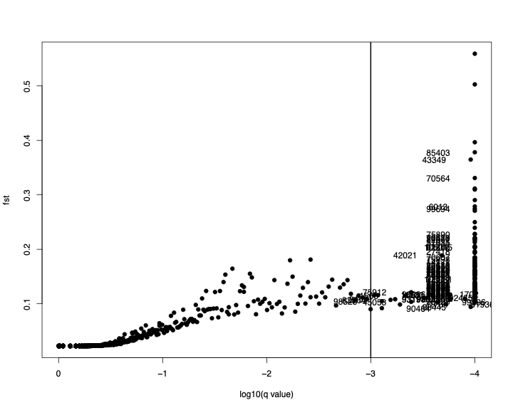
Bayescan ships with a R script that aids in quickly plotting this data.
Get the script from here:
wget https://github.com/wyoibc/popgen_workshop/tree/master/week5/selection/data/plot_R.rsource("plot_R.r")plot_bayescan("test.baye_fst.txt", FDR=0.001)
$outliers
[1] 1566 1568 1700 1702 3159 3192 6013 6650 6931 12697
[11] 14156 14171 14201 14954 18125 18300 18322 18394 18396 24167
[21] 24395 26773 27418 27423 31272 34814 34830 36086 39272 39876
[31] 39889 39890 39910 42021 42351 43349 43516 43760 43771 43775
[41] 43778 45050 45053 46669 46861 48480 49162 50013 51912 51917
[51] 51920 51936 53114 54009 54544 57035 58556 58559 59329 59877
[61] 59878 61797 66090 66817 70550 70551 70553 70554 70556 70557
[71] 70561 70564 70578 70606 70607 70616 70617 70656 70684 70738
[81] 71234 71265 71646 71734 71796 72584 73227 74211 74218 75864
[91] 75866 75878 75883 75885 75888 75890 75898 75905 75912 75926
[101] 75927 75928 75930 75937 75938 75944 76005 76042 76057 76066
[111] 77901 80748 82861 82866 82964 84287 85403 85513 90464 92350
[121] 92465 92826 93197 93198 93199 93639 93640 94661 96296 97405
[131] 97407 97998 98445 98528 99021 99396 99397 99398 99430 99694
[141] 103772 105015 105025 105030 106061
$nb_outliers
[1] 145wget https://github.com/wyoibc/popgen_workshop/tree/master/week5/selection/data/test_chrpos.baye_fst.txttest2 <- read.table("test_chrpos.baye_fst.txt", header=T)
head(test2)
CHR POS num prob log10PO qval alpha fst
1 10 25550 1 0.00000000 -1000.0000 0.997644 0.0000e+00 0.022319
2 10 25560 2 0.00000000 -1000.0000 0.997640 0.0000e+00 0.022319
3 10 25567 3 0.00000000 -1000.0000 0.997640 0.0000e+00 0.022319
4 10 25597 4 0.00020004 -3.6988 0.994060 1.5625e-04 0.022324
5 10 25600 5 0.00020004 -3.6988 0.994060 -5.8927e-05 0.022318
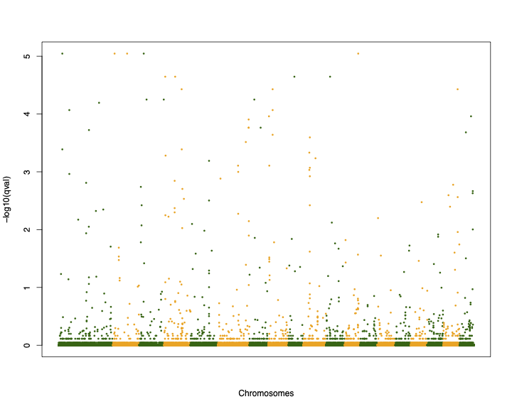
6 10 25602 6 0.00000000 -1000.0000 0.997640 0.0000e+00 0.022319Now let’s draw the Manhattan plot
palette(c("darkgreen", "orange"))

pdf("test_bayescan_mh.pdf", width=10, height=8)

plot(c(1:107309), -log10(test2$qval), col=test2$CHR, pch=16, cex=0.5, xlab="Chromosomes", ylab="-log10(qval)", xaxt='n')

dev.off()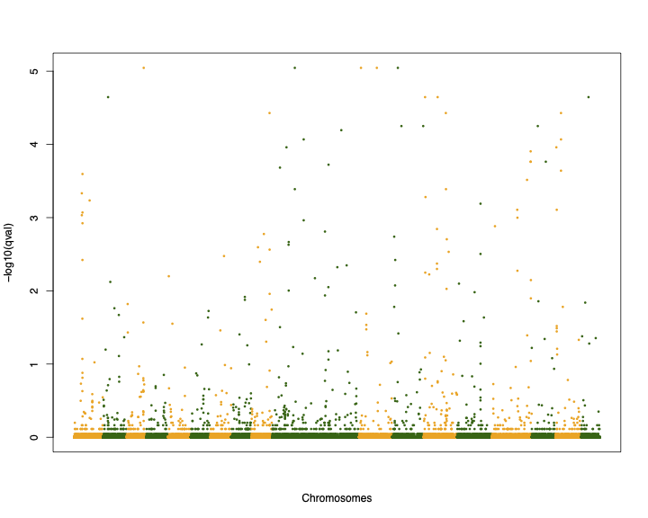
test2_order <- test2[order(test2$CHR),]

palette(c("darkgreen", "orange"))

pdf("test_bayescan_mh_ordered.pdf", width=10, height=8)

plot(c(1:107309), -log10(test2_order$qval), col=test2_order$CHR, pch=16, cex=0.5, xlab="Chromosomes", ylab="-log10(qval)", xaxt='n')

dev.off()