November 12, 2021
So far, we have explored have processed our data to get it from the raw reads that we generally start with into aligned data where our files are now sequences of SNPs or loci that are on a common coordinate system for each individual sample. This allows us to now make inferences based on variation at sites in the alignment across samples. The two types of analyses that we will aim to cover in the final two sessions of the workshop are population structure analysis and inference of selection. We will briefly introduce these conceptually here so that we can dive into these in the coming weeks.
Population assignment is a critical step in many population genetic and phylogeographic studies. Most downstream methods for estimating gene flow, divergence, population size, and other interesting population parameters require populations to be specified by you as inference program input. If you have population structure in your data that you have not adequately accounted for, this can bias many types of analyses. E.g., if you try to estimate the history of population size changes in a group of samples that you assume are a single population when they actually come from multiple discrete populations, this will bias your results.
There are multiple ways to assign individuals to discrete populations. In some cases, you may have a priori ideas about population boundaries based on geographic discontinuities, differences in morphology across a species range, previous genetic data, or other sources of information. However, most of the time you will want to infer the number of populations and population membership of individuals directly from your data. This is essentially a classification problem: we are seeking to classify our whole set of genetic samples into a number of populations, often while also seeking to determine how many populations are present.
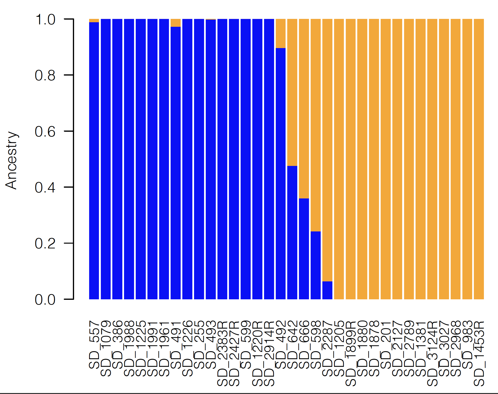
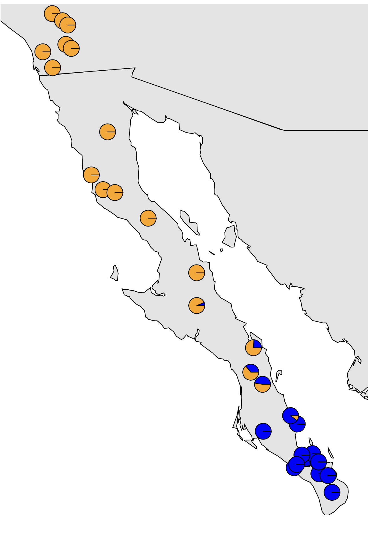
One of the most commonly used programs for the inference of population structure is the aptly named program Structure. Structure is a model-based clustering method that seeks to split individuals into clusters such that linkage disequilibrium is minimized and Hardy-Weinberg equilibrium is maximized within each cluster. Structure us a Bayesian method that relies on Markov chain Monte Carlo (MCMC) sampling, and can thus become somewhat unwieldy with large datasets. Many fast alternatives have been developed since the advent of Structure, including Admixture which utilizes the same model from Structure, but in a faster maximum likelihood implementation. Other alternative approaches do not explicitly model Hardy-Weinberg equilibrium or linkage disequilibrium, including the sNMF appraoch implemented in the LEA R package and DAPC as implemented in the Adegenet R package. All of these methods often produce comparable results, which are often visualized as barplots of the estimated membership of each sample in one or more population clusters or as pie charts of the same information plotted onto a map as show in the figures below.
If using DAPC to estimate population membership, it is important to note that in my experience, with large amounts of data, DAPC is very good at estimating which population a sample belongs to, but if a sample is admixed, it will be confidently placed into the population that it shares the most ancestry with. Barplots or pie charts of DAPC reflect the uncertainty in classification rather than amount of admixture, so care should be taken not to interpret DAPC plots the same way as plots from Strucure, Admixture, sNMF, etc.
An additional critical consideration is that continuous spatial genetic structure across the range of a population can be highly problematic for population structure methods. One of the most common types of continuous spatial structure is isolation by distance (IBD), which occurs when dispersal is limited and individuals that are geographically closer are more related than individuals that are geographically distant. If IBD is strong enough, population structure methods can incorrectly infer the presence of multiple discrete populations with a gradient of admixture between the farthest individuals. This problem is reviewed well in Bradburd et al. 2018 and they developed the method conStruct to simultaneously continuous and discrete spatial structure. The program can be finicky, particularly with regards to missing data, so we won’t use it in the workshop, but it is a powerful tool. In any case, testing to isolation by distance and being aware of its potentially misleading effects can help to prevent incorrect inferences of population structure.
One of the foremost goals in biology is to identify genetic variation underlying traits of interest. Data from population genomic studies offers a unique way of identifying regions of the genome that might control a given trait. For example, consider two populations of a species inhabiting two different environments. It is likely that these population have the greatest fitness in their home environments stemming from genetic adaptations they may have developed to their native conditions. Signatures of these adaptations show up as genomic regions of increased divergence (e.g. higher FST than genomic average) between the populations. Identifying these genomic regions is crucial to our quest of linking phenotypes to genotypes.
Over the years, a number of methods have been developed to identify regions of genomes under Darwinian natural selection. These methods fall into two main categories:
Frequentist methods use only genomic data to identify extreme allele frequency differences between populations. e.g. Bayescan and XTX (Coop et al)
Environmental correlation methods try to identify relationship between environmental differences and genomic differences. e.g. Bayenv (Coop et al) and LFMM (Latent Factor Mixed Models).
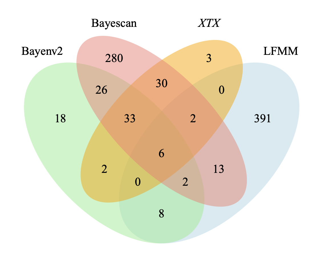
In the final session of this workshop, we will use two of these methods (Bayescan and Bayenv) to identify candidate genes (those likely under natural selection) in the rattlesnake genome. We will compare and contrast results from these two tests to increase our confidence in the inference of natural selection. The goal is to make a venn diagram showing shared and unique candidates as shown in the following figure: